Data Stream Classification Methods
Every few thousand instances, labels flip. Not because reality changed, but because an adversary is poisoning the stream. This is what adversarial data stream classification looks like: a model trying to learn from data it can’t fully trust, where the ground truth itself is occasionally wrong.
This project evaluated five classifiers across seven datasets: synthetic streams with and without adversarial label-flipping, streams with abrupt concept drift, and real-world spam and electricity data. The results split into three tiers of problem difficulty.
Datasets and Methodology
Datasets
-
Synthetic Datasets:
- AGRAWALGenerator: 100,000 instances.
- SEAGenerator: 100,000 instances, plus a drift variant with three abrupt drift points at 25,000, 50,000, and 75,000 instances.
-
Real Datasets:
- Spam Dataset
- Electricity (Elec) Dataset
For synthetic datasets, adversarial attacks were simulated by flipping labels:
- 40,000 to 40,500 instances: 10% labels flipped.
- 60,000 to 60,500 instances: 20% labels flipped.
Classification Models
- Adaptive Random Forest (ARF)
- Streaming Agnostic Model with k-Nearest Neighbors (SAM-kNN)
- Dynamic Weighted Majority (DWM)
- Custom Ensemble (CE) using HoeffdingTreeClassifier
- Robust Custom Ensemble (RCE) using HoeffdingTreeClassifier with drift and adversarial attack detection.
Results
All models were evaluated using Interleaved Test-Then-Train: each instance is tested before being used for training, giving a running accuracy estimate without a separate held-out set. Prequential accuracy (sliding window of 1,000 instances) makes drift events and attack windows visible in the plots.
Overall Accuracy
| Dataset | Model | Overall Accuracy |
|---|---|---|
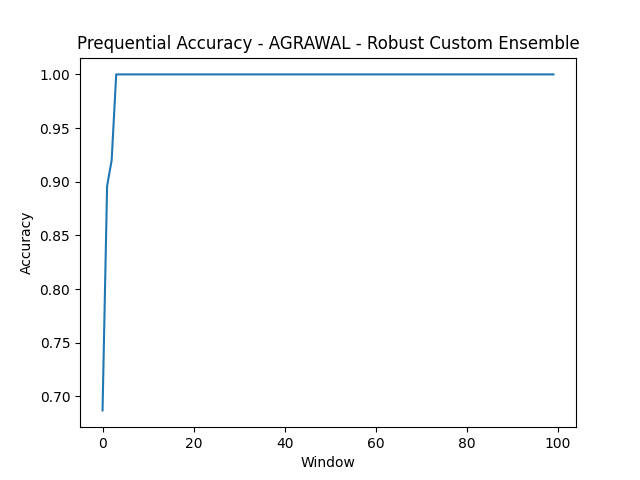
| AGRAWAL | RCE | 0.9950 |
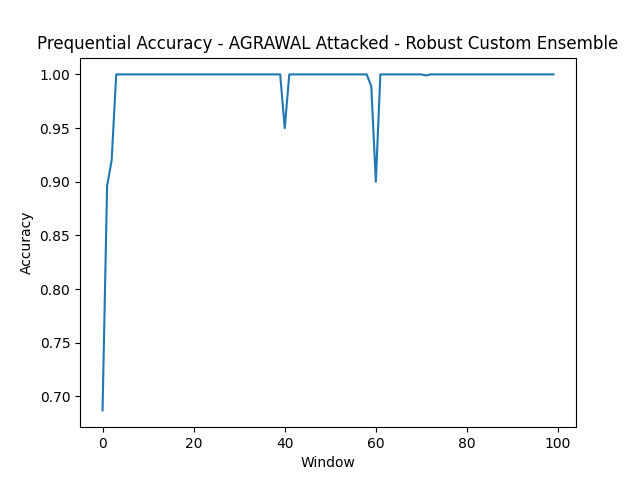
| AGRAWAL Attacked | RCE | 0.9934 |
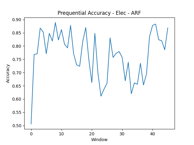
| Electricity | ARF | 0.7664 |
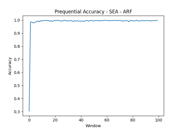
| SEA | ARF | 0.9880 |
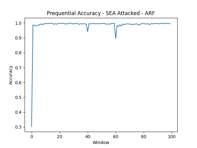
| SEA Attacked | ARF | 0.9848 |
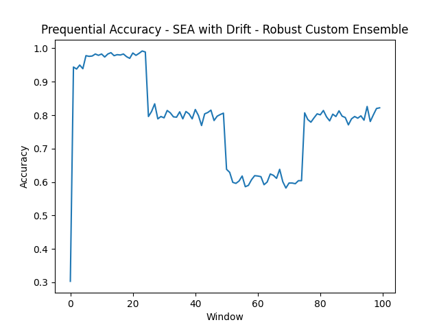
| SEA with Drift | RCE | 0.7885 |
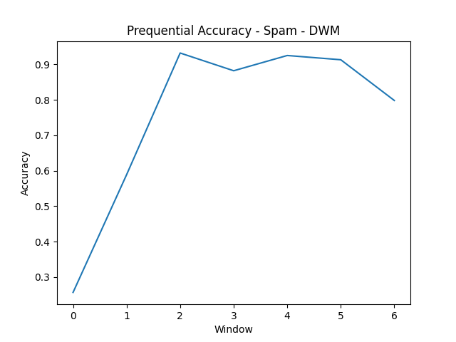
| Spam | DWM | 0.7566 |
Full accuracy details for all models are in Appendix A.
Prequential Accuracy Plots
Prequential accuracy, calculated using a sliding window of 1,000 data instances, gives a dynamic view of model performance over time.
- AGRAWAL
- AGRAWAL Attacked
- Electricity
- SEA
- SEA Attacked
- SEA with Drift
- Spam
Analysis
Three Tiers of Difficulty
The AGRAWAL and SEA synthetic datasets are the easy tier. Both RCE and ARF clear 99% accuracy because the underlying concepts are stable and well-separated. Even under adversarial attack (10% label flipping at instance 40,000, 20% at 60,000), both models hold up. The prequential accuracy plots show brief dips at attack windows followed by recovery within a few hundred instances.
Adversarial attacks are easier to handle than concept drift. This is the most interesting finding. Label flipping is statistical noise that ensemble methods average out; corrupted labels are outvoted by the uncorrupted majority. Concept drift is fundamentally harder: it changes the decision boundary, and no amount of ensemble voting recovers a boundary that’s no longer correct. The SEA drift dataset, with three abrupt drift points at 25k, 50k, and 75k instances, drops RCE to 78.85%, its worst result despite being one of the “simpler” datasets in other conditions.
The real datasets (Electricity at 76.64% for ARF; Spam at 75.66% for DWM) are harder than any synthetic condition. Real concept drift is messier than labeled abrupt transitions. The Electricity prequential accuracy plot shows extended periods of poor performance followed by recovery; the model falls behind during volatile windows and catches up as the concept stabilizes.
SAM-kNN consistently underperforms on clean synthetic data (64% on AGRAWAL) while holding up better on drift and real datasets. Lazy learning adapts locally rather than globally: bad for clean synthetic data where a stable global model would dominate, but more forgiving when the concept drifts unpredictably.
CE vs. RCE
RCE makes one structural change: it monitors agreement between the ensemble’s predictions and incoming labels, flags windows where disagreement exceeds a threshold, and down-weights those instances during training.
On attacked datasets, this works. RCE beats CE on every attacked dataset. On clean data, the detection mechanism correctly identifies no adversarial windows and stays out of the way; accuracy difference between CE and RCE on unattacked streams is negligible.
The limitation is a fixed detection threshold. A sophisticated adversary who knows the threshold could stay just below it indefinitely. Real adversarial robustness needs adaptive detection, not a static heuristic. But for the attack intensities tested here (10-20% label corruption over fixed windows), the approach holds up.
Appendix A
Overall accuracies of all datasets and models:
- AGRAWAL: ARF (0.9943), CE (0.9950), DWM (0.8716), RCE (0.9950), SAM-kNN (0.6641)
- AGRAWAL Attacked: ARF (0.9906), CE (0.9813), DWM (0.8702), RCE (0.9934), SAM-kNN (0.6635)
- Electricity: ARF (0.7664), CE (0.7512), DWM (0.7439), RCE (0.7512), SAM-kNN (0.6677)
- SEA: ARF (0.9880), CE (0.9812), DWM (0.9380), RCE (0.9812), SAM-kNN (0.9752)
- SEA Attacked: ARF (0.9848), CE (0.9581), DWM (0.9372), RCE (0.9791), SAM-kNN (0.9737)
- SEA with Drift: ARF (0.7872), CE (0.7325), DWM (0.7673), RCE (0.7885), SAM-kNN (0.7648)
- Spam: ARF (0.7429), CE (0.7053), DWM (0.7566), RCE (0.7053), SAM-kNN (0.7191)