Applied Statistics for Logistics, Manufacturing, and Training

OLS regression, two-way ANOVA, Poisson probability, and two-sample hypothesis testing applied to logistics economics, manufacturing process control, and workforce training. Each analysis follows the same loop: verify assumptions, fit the model, interpret the output, run diagnostics. All computation in MATLAB.

European Logistics Expenditure via OLS

The premise was simple. Given GDP data for 11 European countries, build a linear model that predicts national logistics expenditure. The dataset spans nearly two orders of magnitude, from Ireland at $33.9B GDP to Germany at $1.19T.

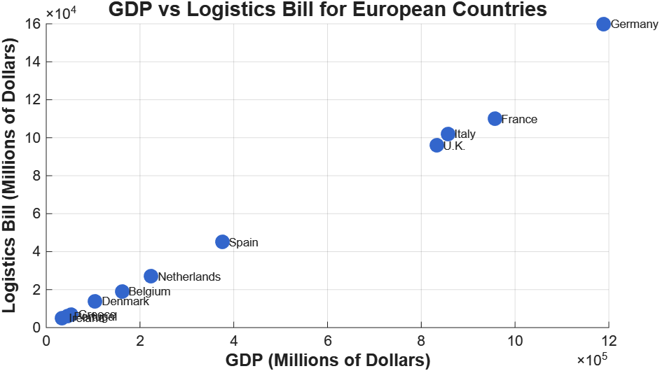
Logistics spending scales with GDP, which is what you’d expect. The OLS fit:

$$\text{Logistics Bill} = -727.56 + 0.124 \times \text{GDP}$$

For every $1B increase in GDP, logistics expenditure rises by ~$124M. R² = 0.9896, which is unusually high for cross-sectional economic data. The F-statistic of 852.28 (p < 0.001) confirms the model is significant.

For a GDP of $600B, the predicted logistics bill is $73.6B, with a 95% prediction interval of [$59.8B, $87.4B]. That $27.6B width is just the reality of n = 11.

Diagnostics

The residuals-vs-fitted plot tells a different story than R² alone.

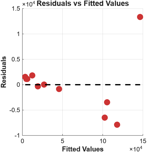
Residuals cluster tightly for small fitted values, swing negative in the mid-range, then one large positive residual appears at the extreme. That’s Germany. As Europe’s largest logistics hub, with extensive transit infrastructure and a disproportionate share of continental freight, Germany generates logistics spending that exceeds what a GDP-based model would predict. It acts as a high-leverage point that pulls the regression line toward it while simultaneously violating it.

I ran the sensitivity analysis: removing Germany improved RMSE by 81%. The model without Germany still holds, but the coefficient shifts, confirming that one country was exerting substantial influence on the parameter estimates. This doesn’t mean Germany should be excluded. It means a logistics-specific predictor (freight volume, port throughput) would capture variation that GDP alone can’t.

Testing H₀: β₀ = 0 yields t = -0.285, p = 0.782. The non-significant intercept makes economic sense: a country with zero GDP should have zero logistics expenditure.

Line Speed and Carbonation: Two-Way ANOVA

A bottling line runs at four speeds (210, 240, 270, 300 bpm) with two carbonation levels (10%, 12%). Five replicates per combination, 40 observations total. The question: does line speed affect fill accuracy, and do the two factors interact?

Before touching the ANOVA, I checked both assumptions.

Normality: chi-square goodness-of-fit yields χ² = 1.026, df = 4, p = 0.9058. Consistent with normality.

Homogeneity of variance: Levene’s test, F = 1.6935, p = 0.1460. Variances not significantly different across groups. Both hold.

Source	SS	df	MS	F	p-value
Line Speed	21.875	3	7.292	4.934	0.0063
Carbonation	0.812	1	0.812	0.550	0.4639
Interaction	0.039	3	0.013	0.009	0.9989
Error	47.288	32	1.478	—	—

Line speed is significant (F = 4.934, p = 0.0063). Carbonation is not (p = 0.4639). The interaction is essentially zero.

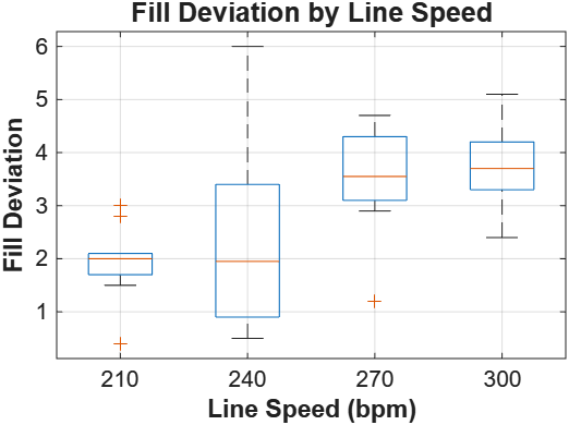
210 bpm produces the lowest fill deviations with the tightest spread. Both median and variance increase with speed. Post-hoc Tukey HSD confirms 210 bpm is significantly different from 270 and 300 bpm.

An interaction p-value of 0.9989

That’s about as close to 1 as you’ll see in practice. The effect of line speed on fill deviation is identical regardless of carbonation level.

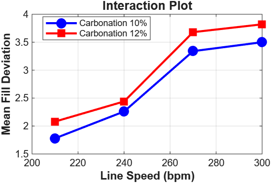
In practice this means the two factors can be optimised independently. You don’t need to recalibrate speed settings every time the carbonation recipe changes.

Poisson Breakdowns

Same manufacturing setting, different question. Breakdowns occur at λ = 1.5 per 8-hour shift. The Poisson model handles discrete events at a constant rate within a fixed interval, assuming independence between events.

The key probabilities:

• P(X = 2) per shift: 0.2510
• P(X < 2) per shift: 0.5578
• P(X = 0) across three consecutive shifts: 0.0111

Over a 24-hour day, there’s a 98.9% probability of at least one breakdown. Maintenance needs to cover all shifts, not just days. Parts inventory should be sized for roughly 30 breakdowns per week (21 shifts at λ = 1.5).

A 20% reduction in breakdown rate to λ = 1.2 (achievable through preventive maintenance) drops the 3-shift expected count from 4.5 to 3.6. These improvements compound. The probability of a completely breakdown-free day goes from 1.1% to 2.7%.

The model assumes constant rate, independence, and stationarity. Operator fatigue, equipment degradation over time, seasonal variation, all of these could violate those assumptions. In practice you’d track observed counts against Poisson predictions and update λ when they diverge.

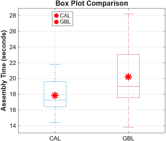
Welch’s t-Test: CAL vs GBL

Two training methods for assembly tasks: Computer Assisted Learning (CAL) and Group-Based Learning (GBL). Twelve employees per group. Does CAL produce faster assembly times?

Statistic	CAL	GBL
Mean	17.850s	20.217s
Std Dev	2.345s	4.421s
Range	[14.4, 21.8]	[13.8, 28.2]

CAL has a 2.367-second advantage and roughly four times lower variance.

An F-test for equal variances returns F = 0.281, p = 0.046. The variances are significantly different. This rules out the standard pooled t-test and requires Welch’s, which uses separate variance estimates and applies the Welch-Satterthwaite approximation for degrees of freedom. Running the pooled version here would produce results on a violated assumption.

Results:

• t-statistic: -1.6384
• Degrees of freedom: 16.74 (Welch-Satterthwaite)
• p-value (one-tailed): 0.0600
• Critical value (α = 0.05): -1.7412

We fail to reject H₀. At the 5% level, there’s insufficient evidence to conclude CAL is faster.

But p = 0.06 sitting just above the threshold, on n = 12 per group with a variance ratio of 4:1, doesn’t mean the effect isn’t real. The 2.4-second improvement (11.7%) could easily be practically meaningful in a setting where seconds accumulate across thousands of units per day. The test simply doesn’t have enough power to distinguish a moderate effect from noise at this sample size. A power analysis would point to 20-30 subjects per group to reliably detect an effect this size.

The result is better described as inconclusive than negative. That distinction matters if someone is making a training decision based on it.

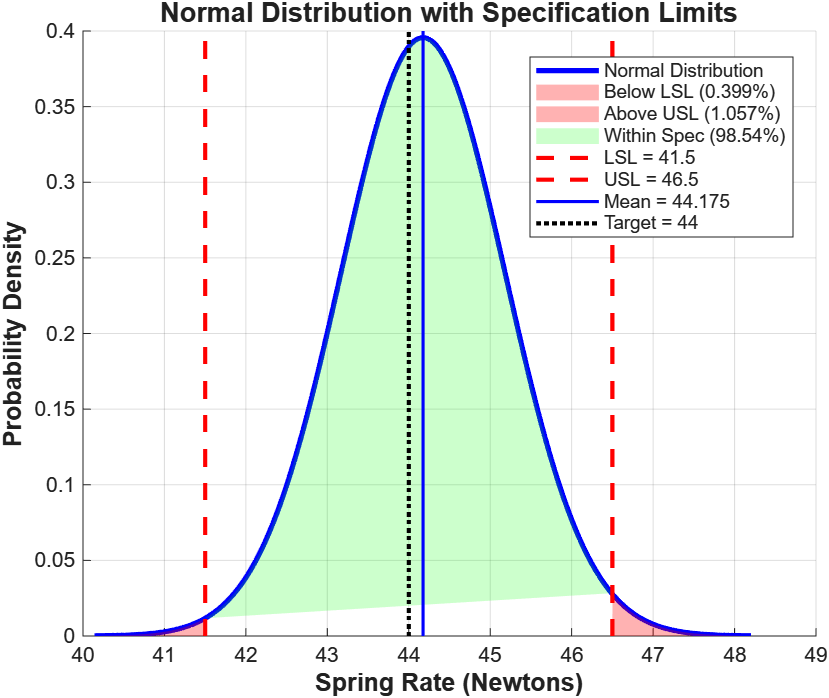
Spring Rate Analysis

100 springs, sample mean 44.175 N, standard deviation 1.008 N, specification limits 41.5 N (LSL) to 46.5 N (USL), target 44 N.

Converting to z-scores:

• z_lower = (41.5 - 44.175) / 1.008 = -2.653
• z_upper = (46.5 - 44.175) / 1.008 = 2.306

98.54% of springs within spec. 0.40% below LSL, 1.06% above USL. The asymmetry (more failing above than below) reflects the process mean sitting 0.175 N above target.

Is the process centered? One-sample t-test for H₀: μ = 44 N:

• t(99) = 1.735
• p-value (two-tailed) = 0.0858

We fail to reject. The 0.175 N offset could plausibly arise from sampling variability alone. The 95% confidence interval [43.975, 44.375] N contains the target.

The process is both capable (98.5% within spec) and centered (mean not significantly different from target). The 6σ spread of 6.048 N fits inside the 5 N specification window, but not with a lot of margin. Any upward drift in process variability needs to be caught early.

What the Diagnostics Actually Did

In the GDP regression, the residual plot exposed Germany’s influence on the parameter estimates in a way that R² = 0.99 completely masked. In the training comparison, the F-test for equal variances shifted the analysis from a pooled t-test to Welch’s, cutting the degrees of freedom from 22 to 16.74 and changing what conclusions were defensible.

Skipping the assumption checks would have left both of those points invisible. The models would have fit, the p-values would have looked clean, and the conclusions would have been subtly wrong.